Chopping and nodding in Scopesim
This notebook demonstrates how to use the ChopNod effect in Scopesim. Both chopping and nodding are currently defined as two-point patterns, where the throw direction is given as a 2D vector (dx, dy) in metis['chop_nod'].meta['chop_offsets'] and metis['chop_nod'].meta['nod_offsets']. For parallel nodding, the two vectors are parallel (typically nod_offset = - chop_offset, giving a three-point pattern), for perpendicular nodding, the vectors are orthogonal.
[1]:
import scopesim as sim
sim.bug_report()

# Edit this path if you have a custom install directory, otherwise comment it out.
sim.rc.__config__["!SIM.file.local_packages_path"] = "../../../../"
Python:
 3.9.7 (default, Sep 28 2021, 17:45:03)
[GCC 9.3.0]

scopesim :  0.4.0
numpy :  1.22.3
scipy :  1.8.0
astropy :  5.0.1
matplotlib :  3.5.1
synphot :  1.1.1
skycalc_ipy : version number not available
requests :  2.27.1
bs4 :  4.10.0
yaml :  6.0

Operating system:  Linux
         Release:  5.11.0-1019-aws
         Version:  #20~20.04.1-Ubuntu SMP Tue Sep 21 10:40:39 UTC 2021
         Machine:  x86_64
[2]:
from matplotlib import pyplot as plt
%matplotlib inline
If you haven’t got the instrument packages yet, uncomment the following cell.
[3]:
# sim.download_package(["instruments/METIS", "telescopes/ELT", "locations/Armazones"])
[4]:
cmd = sim.UserCommands(use_instrument="METIS", set_modes=['img_n'])
[5]:
metis = sim.OpticalTrain(cmd)
metis['chop_nod'].include = True
The default is perpendicular nodding, with the chop throw in the x-direction and the nod throw in the y direction.
[6]:
print("Chop offsets:", sim.utils.from_currsys(metis['chop_nod'].meta['chop_offsets']))
print("Nod offsets: ", sim.utils.from_currsys(metis['chop_nod'].meta['nod_offsets']))
Chop offsets: [3, 0]
Nod offsets:  [0, 3]
[7]:
src = sim.source.source_templates.star()
[8]:
metis.observe(src, update=True)
imghdu = metis.readout()[0][1]
Requested exposure time: 1.000 s
Warning: The detector will be saturated!
Exposure parameters:
                DIT: 0.011 s  NDIT: 90
Total exposure time: 0.990 s
[9]:
plt.imshow(imghdu.data, origin='lower', vmin=-5e7, vmax=5e7)
plt.colorbar()
[9]:
<matplotlib.colorbar.Colorbar at 0x7f776b752b20>
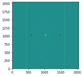
For parallel nodding, turn the nod throw into the x-direction as well.
[10]:
metis['chop_nod'].meta['nod_offsets'] = [-3, 0]
[11]:
imghdu_par = metis.readout()[0][1]
Requested exposure time: 1.000 s
Warning: The detector will be saturated!
Exposure parameters:
                DIT: 0.011 s  NDIT: 90
Total exposure time: 0.990 s
[12]:
plt.imshow(imghdu_par.data, origin='lower', vmin=-5e7, vmax=5e7)
[12]:
<matplotlib.image.AxesImage at 0x7f776b703fd0>
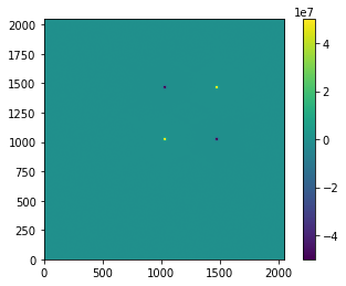
Other four-point patterns are possible:
[13]:
metis['chop_nod'].meta['nod_offsets'] = [-3, 3]
imghdu_3 = metis.readout()[0][1]
plt.imshow(imghdu_3.data, origin='lower', vmin=-5e7, vmax=5e7)
Requested exposure time: 1.000 s
Warning: The detector will be saturated!
Exposure parameters:
                DIT: 0.011 s  NDIT: 90
Total exposure time: 0.990 s
[13]:
<matplotlib.image.AxesImage at 0x7f77587ad580>

[14]:
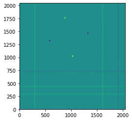
metis['chop_nod'].meta['chop_offsets'] = [-3, 2]
metis['chop_nod'].meta['nod_offsets'] = [2, 3]
imghdu_4 = metis.readout()[0][1]
plt.imshow(imghdu_4.data, origin='lower', vmin=-5e7, vmax=5e7)
Requested exposure time: 1.000 s
Warning: The detector will be saturated!
Exposure parameters:
                DIT: 0.011 s  NDIT: 90
Total exposure time: 0.990 s
[14]:
<matplotlib.image.AxesImage at 0x7f775671f760>