This notebook demonstrates the effect detector_readout_parameters, which selects between the different detector readout modes. These are fast and slow for the HAWAII2RG detectors, and high_capacity and low_capacity for the Geosnap detector.
[1]:
import os
import numpy as np
from astropy import units as u
from matplotlib import pyplot as plt
from matplotlib.colors import LogNorm
%matplotlib inline
[2]:
import scopesim as sim
from scopesim.utils import from_currsys
sim.bug_report()

# Edit this path if you have a custom install directory, otherwise comment it out.
sim.rc.__config__["!SIM.file.local_packages_path"] = "../../../../"
Python:
 3.9.7 (default, Sep 28 2021, 17:45:03)
[GCC 9.3.0]

scopesim :  0.4.0
numpy :  1.22.3
scipy :  1.8.0
astropy :  5.0.1
matplotlib :  3.5.1
synphot :  1.1.1
skycalc_ipy : version number not available
requests :  2.27.1
bs4 :  4.10.0
yaml :  6.0

Operating system:  Linux
         Release:  5.11.0-1019-aws
         Version:  #20~20.04.1-Ubuntu SMP Tue Sep 21 10:40:39 UTC 2021
         Machine:  x86_64
If you haven’t got the instrument packages yet, uncomment the following cell.
[3]:
# sim.download_package(['instruments/METIS', 'telescopes/ELT', 'locations/Armazones'])
[4]:
cmd = sim.UserCommands(use_instrument="METIS", set_modes=["img_lm"])
The default readout mode for img_lm is the fast mode:
[5]:
cmd["!OBS.detector_readout_mode"]
[5]:
'fast'
We build the optical train using the default mode, and then check that the relevant parameters (mindit, full_well, readout_noise and dark_current) are taken over correctly, first in the cmds property of the optical train, then - most importantly - into the parameters of the affected Effect objects (demonstrated for the readout_noise effect).
[6]:
metis = sim.OpticalTrain(cmd)
[7]:
metis.cmds["!DET"]
[7]:
{'detector': 'HAWAII2RG',
 'image_plane_id': 0,
 'temperature': -230,
 'dit': '!OBS.dit',
 'ndit': '!OBS.ndit',
 'layout': {'file_name': 'FPA_metis_img_lm_layout.dat'},
 'qe_curve': {'file_name': 'QE_detector_H2RG_METIS.dat'},
 'linearity': {'file_name': 'FPA_linearity_HxRG.dat'},
 'element_name': 'METIS_DET_IMG_LM',
 'mindit': 0.04,
 'full_well': 100000.0,
 'readout_noise': 70,
 'dark_current': 0.05}
[8]:
from_currsys(metis['readout_noise'].meta['noise_std'])
[8]:
70
At this stage, we have access to the available detector modes and the parameter values that are set by them:
[9]:
print(metis['detector_readout_parameters'].list_modes())
fast:
  description: HAWAII2RG, fast mode
  !DET.mindit: 0.04
  !DET.full_well: 100000.0
  !DET.readout_noise: 70
  !DET.dark_current: 0.05
slow:
  description: HAWAII2RG, slow mode
  !DET.mindit: 1.3
  !DET.full_well: 100000.0
  !DET.readout_noise: 15
  !DET.dark_current: 0.05
We can switch to the slow mode in the existing optical train by doing
[10]:
metis.cmds["!OBS.detector_readout_mode"] = "slow"
metis.update()
[11]:
metis.cmds["!DET"]
[11]:
{'detector': 'HAWAII2RG',
 'image_plane_id': 0,
 'temperature': -230,
 'dit': '!OBS.dit',
 'ndit': '!OBS.ndit',
 'layout': {'file_name': 'FPA_metis_img_lm_layout.dat'},
 'qe_curve': {'file_name': 'QE_detector_H2RG_METIS.dat'},
 'linearity': {'file_name': 'FPA_linearity_HxRG.dat'},
 'element_name': 'METIS_DET_IMG_LM',
 'mindit': 1.3,
 'full_well': 100000.0,
 'readout_noise': 15,
 'dark_current': 0.05}
[12]:
from_currsys(metis['readout_noise'].meta['noise_std'])
[12]:
15
Test: detector noise level (LSS-L)
To investigate the behaviour of the detector readout modes, we look at the L-band long-slit mode where the areas of the detector outside the spectral trace contain only readout noise and dark current. The default mode for long-slit spectroscopy is the slow mode, and we’ll switch to the fast mode afterwards.
[13]:
sky = sim.source.source_templates.empty_sky()
[14]:
cmd = sim.UserCommands(use_instrument="METIS", set_modes="lss_l",
                      properties={"!OBS.exptime": 1000})
metis = sim.OpticalTrain(cmd)
[15]:
print("Detector mode:", metis.cmds["!OBS.detector_readout_mode"])
metis.observe(sky, update=True)
hdul_slow = metis.readout()[0]
Detector mode: slow
Requested exposure time: 1000.000 s
Exposure parameters:
                DIT: 6.024 s  NDIT: 166
Total exposure time: 1000.000 s
We get the statistics in a strip at the left edge of the detector that is not covered by any source or background flux and compare to the expected values.
[16]:
ndit_slow = from_currsys("!OBS.ndit")
dit_slow = from_currsys("!OBS.dit")

bg_slow = hdul_slow[1].data[250:1750, 10:200].mean()
bg_slow_expected = dit_slow * ndit_slow * from_currsys("!DET.dark_current")

noise_slow = hdul_slow[1].data[250:1750, 10:200].std()
noise_slow_expected = np.sqrt(ndit_slow) * from_currsys("!DET.readout_noise")
Do the same for the fast mode.
[17]:
hdul_fast = metis.readout(detector_readout_mode="fast")[0]
Requested exposure time: 1000.000 s
Exposure parameters:
                DIT: 6.024 s  NDIT: 166
Total exposure time: 1000.000 s
[18]:
ndit_fast = from_currsys("!OBS.ndit")
dit_fast = from_currsys("!OBS.dit")

bg_fast = hdul_fast[1].data[250:1750, 10:200].mean()
bg_fast_expected = dit_fast * ndit_fast * from_currsys("!DET.dark_current")

noise_fast = hdul_fast[1].data[250:1750, 10:200].std()
noise_fast_expected = np.sqrt(ndit_fast) * from_currsys("!DET.readout_noise")
[19]:
print(f"""
Fast: ndit  = {ndit_fast}
      bg    = {bg_fast:5.1f}  expected: {bg_fast_expected:5.1f}
      noise = {noise_fast:5.1f}  expected: {noise_fast_expected:5.1f}""")
print(f"""
Slow: ndit  = {ndit_slow}
      bg    = {bg_slow:5.1f}  expected: {bg_slow_expected:5.1f}
      noise = {noise_slow:5.1f}  expected: {noise_slow_expected:.1f}""")
Fast: ndit  = 166
      bg    =  49.3  expected:  50.0
      noise = 902.5  expected: 901.9

Slow: ndit  = 166
      bg    =  50.1  expected:  50.0
      noise = 193.6  expected: 193.3
Finally, we can let Scopesim automatically select the “best” mode.
[20]:
hdul_auto = metis.readout(detector_readout_mode="auto")[0]
Detector mode set to slow
Requested exposure time: 1000.000 s
Exposure parameters:
                DIT: 6.024 s  NDIT: 166
Total exposure time: 1000.000 s
Test: Full well (IMG-N)
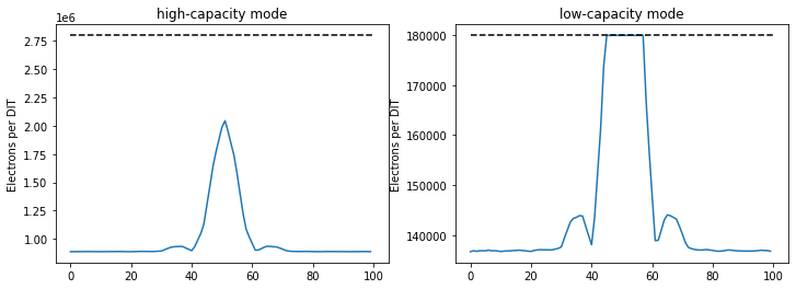
This demonstrates the high- and low-capacity modes of the Geosnap detector. The setup uses a neutral-density filter to ensure that the background does not saturate the detector in the low-capacity mode. The source is a very bright star, which saturates in the low-capacity mode but does not in the high-capacity mode.
[21]:
star = sim.source.source_templates.star(flux=20 * u.Jy)
[22]:
cmd_n = sim.UserCommands(use_instrument="METIS", set_modes=['img_n'],
                        properties={"!OBS.filter_name": "N2", "!OBS.nd_filter_name": "ND_OD1"})
metis_n = sim.OpticalTrain(cmd_n)
[23]:
metis_n.observe(star, update=True)
print("--- high-capacity mode ---")
hdul_high = metis_n.readout(detector_readout_mode="high_capacity")[0]
fullwell_high = from_currsys("!DET.full_well")
ndit_high = from_currsys("!OBS.ndit")
print("--- low-capacity mode ---")
hdul_low = metis_n.readout(detector_readout_mode="low_capacity")[0]
ndit_low = from_currsys("!OBS.ndit")
fullwell_low = from_currsys("!DET.full_well")
--- high-capacity mode ---
Requested exposure time: 1.000 s
Exposure parameters:
                DIT: 0.071 s  NDIT: 14
Total exposure time: 1.000 s
--- low-capacity mode ---
Requested exposure time: 1.000 s
Warning: The detector will be saturated!
Exposure parameters:
                DIT: 0.011 s  NDIT: 90
Total exposure time: 0.990 s
[24]:
detimg_high = hdul_high[1].data / ndit_high
detimg_low = hdul_low[1].data / ndit_low
[25]:
plt.figure(figsize=(12, 4))
plt.subplot(121)
plt.plot(detimg_high[1024, 974:1074])
plt.title("high-capacity mode")
plt.hlines(fullwell_high, 0, 100, colors='k', linestyles='dashed')
plt.ylabel("Electrons per DIT")

plt.subplot(122)
plt.plot(detimg_low[1024, 974:1074])
plt.title(label="low-capacity mode")
plt.hlines(fullwell_low, 0, 100, colors='k', linestyles="dashed")
plt.ylabel("Electrons per DIT")
[25]:
Text(0, 0.5, 'Electrons per DIT')