This notebook demonstrates the use of the FilterWheel in Scopesim. The METIS configuration contains two instances of this effect, named filter_wheel (for science filters) and nd_filter_wheel (for neutral-density filters). Each filter wheel contains a number of predefined filters, with different filter sets for the LM- and N-band imagers.
[1]:
import numpy as np
from matplotlib import pyplot as plt
from matplotlib.colors import LogNorm
%matplotlib inline
[2]:
import scopesim as sim
sim.bug_report()

# Edit this path if you have a custom install directory, otherwise comment it out.
sim.rc.__config__["!SIM.file.local_packages_path"] = "../../../../"
Python:
 3.9.7 (default, Sep 28 2021, 17:45:03)
[GCC 9.3.0]

scopesim :  0.4.0
numpy :  1.22.3
scipy :  1.8.0
astropy :  5.0.1
matplotlib :  3.5.1
synphot :  1.1.1
skycalc_ipy : version number not available
requests :  2.27.1
bs4 :  4.10.0
yaml :  6.0

Operating system:  Linux
         Release:  5.11.0-1019-aws
         Version:  #20~20.04.1-Ubuntu SMP Tue Sep 21 10:40:39 UTC 2021
         Machine:  x86_64
If you haven’t got the instrument packages yet, uncomment the following cell.
[3]:
# sim.download_package(["instruments/METIS", "telescopes/ELT", "locations/Armazones"])
[4]:
cmd = sim.UserCommands(use_instrument="METIS", set_modes=['img_lm'])
The filter to use is defined by setting !OBS.filter_name. In img_lm mode, it defaults to the Lp filter:
[5]:
cmd['!OBS.filter_name']
[5]:
'Lp'
[6]:
metis = sim.OpticalTrain(cmd)
The METIS package defines the list of filters that are available in the real instrument:
[7]:
metis['filter_wheel'].filters
[7]:
{'open': FilterCurve: "open",
 'Lp': FilterCurve: "Lp",
 'short-L': FilterCurve: "short-L",
 'L_spec': FilterCurve: "L_spec",
 'Mp': FilterCurve: "Mp",
 'M_spec': FilterCurve: "M_spec",
 'Br_alpha': FilterCurve: "Br_alpha",
 'Br_alpha_ref': FilterCurve: "Br_alpha_ref",
 'PAH_3.3': FilterCurve: "PAH_3.3",
 'PAH_3.3_ref': FilterCurve: "PAH_3.3_ref",
 'CO_1-0_ice': FilterCurve: "CO_1-0_ice",
 'CO_ref': FilterCurve: "CO_ref",
 'H2O-ice': FilterCurve: "H2O-ice",
 'IB_4.05': FilterCurve: "IB_4.05",
 'HCI_L_short': FilterCurve: "HCI_L_short",
 'HCI_L_long': FilterCurve: "HCI_L_long",
 'HCI_M': FilterCurve: "HCI_M"}
At any moment one of these filters is in the optical path and used for the simulation. Initially, this is the one set by !OBS.filter_name:
[8]:
metis['filter_wheel'].current_filter
[8]:
FilterCurve: "Lp"
The current filter can be changed to any of the filters in the list:
[9]:
metis['filter_wheel'].change_filter("PAH_3.3")
[10]:
metis['filter_wheel'].current_filter
[10]:
FilterCurve: "PAH_3.3"
Observing the same source in different filters
[11]:
src = sim.source.source_templates.empty_sky()
[12]:
metis['filter_wheel'].change_filter("Lp")

metis.observe(src)
img_Lp = metis.image_planes[0].data
[13]:
metis['filter_wheel'].change_filter("PAH_3.3")

metis.observe(src, update=True)
img_PAH = metis.image_planes[0].data
[14]:
print("Background in Lp:      {:8.1f} counts/s".format(np.median(img_Lp)))
print("Background in PAH_3.3: {:8.1f} counts/s".format(np.median(img_PAH)))
Background in Lp:      251483.7 counts/s
Background in PAH_3.3:   8763.5 counts/s
Using the neutral-density filter wheel
METIS also has neutral-density filters that can be inserted and changed using the nd_filter_wheel effect. The transmission of the filter ND_ODx is \(10^{-x}\).
[15]:
metis['nd_filter_wheel'].filters
[15]:
{'open': FilterCurve: "open",
 'ND_OD1': FilterCurve: "ND_OD1",
 'ND_OD2': FilterCurve: "ND_OD2",
 'ND_OD3': FilterCurve: "ND_OD3",
 'ND_OD4': FilterCurve: "ND_OD4",
 'ND_OD5': FilterCurve: "ND_OD5"}
[16]:
metis['nd_filter_wheel'].current_filter
[16]:
FilterCurve: "open"
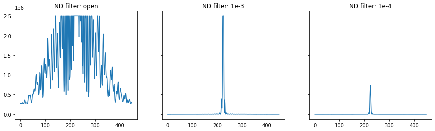
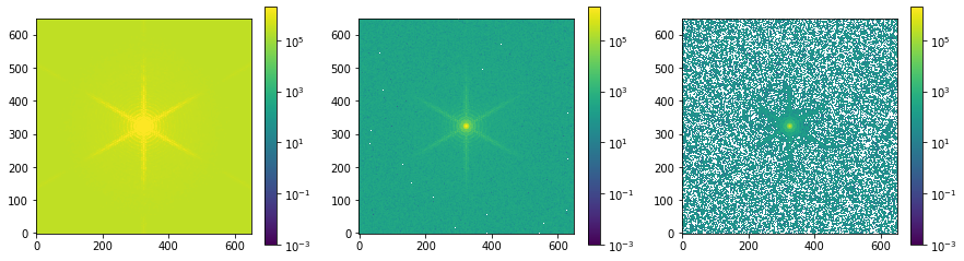
Observe a bright star (default arguments result in Vega at 0 mag) in the Lp filter. It will be found that the star saturates the detector in the open position, and requires the ND_OD4 filter not to do so.
[17]:
star = sim.source.source_templates.star()
[18]:
metis['filter_wheel'].change_filter('Lp')
[19]:
metis['nd_filter_wheel'].change_filter("open")
metis.observe(star, update=True)
hdu_open = metis.readout()[0][1]
Requested exposure time: 1.000 s
Warning: The detector will be saturated!
Exposure parameters:
                DIT: 0.040 s  NDIT: 25
Total exposure time: 1.000 s
[20]:
metis['nd_filter_wheel'].change_filter("ND_OD3")
metis.observe(star, update=True)
hdu_OD3 = metis.readout()[0][1]
Requested exposure time: 1.000 s
Warning: The detector will be saturated!
Exposure parameters:
                DIT: 0.040 s  NDIT: 25
Total exposure time: 1.000 s
[21]:
metis['nd_filter_wheel'].change_filter("ND_OD4")
metis.observe(star, update=True)
hdu_OD4 = metis.readout()[0][1]
Requested exposure time: 1.000 s
Exposure parameters:
                DIT: 0.091 s  NDIT: 11
Total exposure time: 1.000 s
[22]:
plt.figure(figsize=(15, 4))
plt.subplot(131)
plt.imshow(hdu_open.data[700:1350, 700:1350], origin='lower', norm=LogNorm(vmin=1e-3, vmax=2e6))
plt.colorbar()
plt.subplot(132)
plt.imshow(hdu_OD3.data[700:1350, 700:1350], origin='lower', norm=LogNorm(vmin=1e-3, vmax=2e6))
plt.colorbar()
plt.subplot(133)
plt.imshow(hdu_OD4.data[700:1350, 700:1350], origin='lower', norm=LogNorm(vmin=1e-3, vmax=2e6))
plt.colorbar()
[22]:
<matplotlib.colorbar.Colorbar at 0x7f78c3b6a1f0>
[23]:
fig, (ax1, ax2, ax3) = plt.subplots(1, 3, sharey=True, figsize=(15, 4))

ax1.plot(hdu_open.data[800:1250, 1024])
ax1.set_title("ND filter: open")
ax2.plot(hdu_OD3.data[800:1250, 1024])
ax2.set_title("ND filter: 1e-3")
ax3.plot(hdu_OD4.data[800:1250, 1024])
ax3.set_title("ND filter: 1e-4")
[23]:
Text(0.5, 1.0, 'ND filter: 1e-4')