This notebook shows the most basic setup for long-slit spectroscopy, using a star as the source.
[1]:
import numpy as np
from matplotlib import pyplot as plt
from matplotlib.colors import LogNorm
%matplotlib inline
[2]:
import scopesim as sim
sim.bug_report()

# Edit this path if you have a custom install directory, otherwise comment it out.
sim.rc.__config__["!SIM.file.local_packages_path"] = "../../../../"
Python:
 3.9.7 (default, Sep 28 2021, 17:45:03)
[GCC 9.3.0]

scopesim :  0.4.0
numpy :  1.22.3
scipy :  1.8.0
astropy :  5.0.1
matplotlib :  3.5.1
synphot :  1.1.1
skycalc_ipy : version number not available
requests :  2.27.1
bs4 :  4.10.0
yaml :  6.0

Operating system:  Linux
         Release:  5.11.0-1019-aws
         Version:  #20~20.04.1-Ubuntu SMP Tue Sep 21 10:40:39 UTC 2021
         Machine:  x86_64
If you haven’t got the instrument packages yet, uncomment the following cell.
[3]:
# sim.download_package(["instruments/METIS", "telescopes/ELT", "locations/Armazones"])
Set up the instrument in lss_l mode:
[4]:
cmd = sim.UserCommands(use_instrument="METIS", set_modes=['lss_l'])
[5]:
metis = sim.OpticalTrain(cmd)
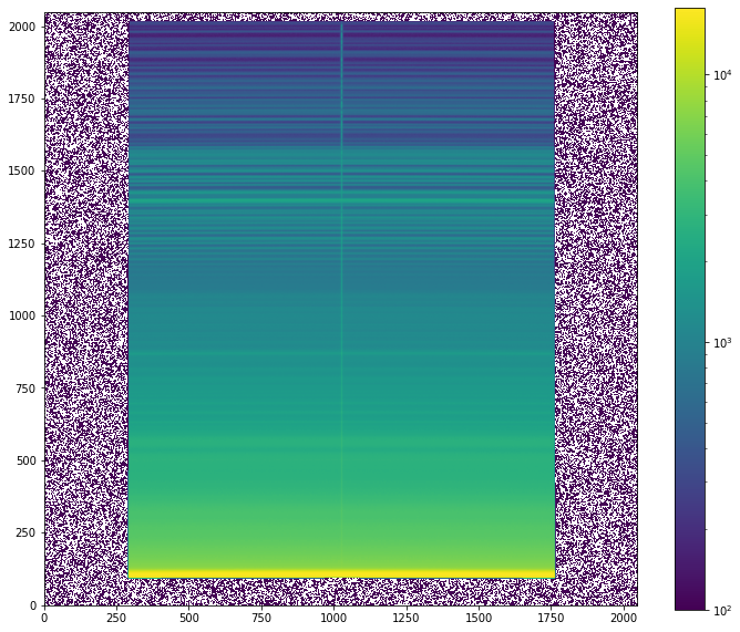
The source is a star with Vega spectrum and apparent brightness of 12 mag.
[6]:
src = sim.source.source_templates.star(flux=12)
[7]:
metis.observe(src, update=True)
result = metis.readout(detector_readout_mode="auto")[0][1]
Detector mode set to slow
Requested exposure time: 1.000 s
    increased to MINDIT: 1.300 s
Exposure parameters:
                DIT: 1.300 s  NDIT: 1
Total exposure time: 1.300 s
[8]:
plt.figure(figsize=(12,10))
plt.imshow(result.data, origin='lower', norm=LogNorm(vmin=100))
plt.colorbar()
[8]:
<matplotlib.colorbar.Colorbar at 0x7faa2956e730>
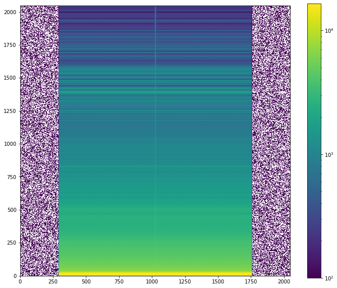
Realistic spectral mapping
The default configuration for METIS applies a mapping of the two-dimensional spectrum onto the detector that is perfectly linear in both the wavelength and spatial directions. The trace definitions for the actual expected mappings are also available. To use them, the parameter !OBS.trace_file needs to be set. The difference is fairly small.
[9]:
cmds = sim.UserCommands(use_instrument="METIS", set_modes=['lss_l'])
cmds['!OBS.trace_file'] = "TRACE_LSS_L.fits"
[10]:
metis = sim.OpticalTrain(cmds)
[11]:
metis.observe(src, update=True)
result_2 = metis.readout()[0][1]
Requested exposure time: 1.000 s
    increased to MINDIT: 1.300 s
Exposure parameters:
                DIT: 1.300 s  NDIT: 1
Total exposure time: 1.300 s
[12]:
plt.figure(figsize=(12,10))
plt.imshow(result_2.data, origin='lower', norm=LogNorm(vmin=100))
plt.colorbar()
[12]:
<matplotlib.colorbar.Colorbar at 0x7faa297bcbb0>