Observing a galaxy with MICADO in wide-field MCAO mode

In this example we will generate a basic galaxy object with the help of the ScopeSim_templates package. We will then create a model of the ELT+MORFEO+MICADO optical system using the MICADO package.

%matplotlib inline
import os
import datetime
import numpy as np
import matplotlib.pyplot as plt
from matplotlib.colors import LogNorm
from astropy import units as u

import scopesim as sim
import scopesim_templates as sim_tp

Download the relevant scopesim instrument packages

We will need the MICADO package, as well as the support packages for Armazones, the ELT, and MORFEO. If you have not yet downloaded the packages, you can use the download_packages command.

sim.download_packages(["Armazones", "ELT", "MORFEO", "MICADO"])

Note

In ScopeSim v0.5 both download_packages (new format) and download_package (old format) exist.

If we would like to keep the instrument packages in a separate directory, we can set the following config value:

sim.rc.__config__["!SIM.file.local_packages_path"] = "path/to/packages"

Set up on-sky source object

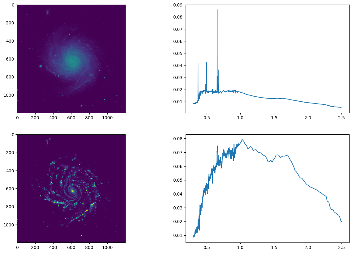
For ease of use we will use the helper function from ScopeSim_templates to create a two-layer spiral galaxy object. The Source object contains two image layers (in <Source>.fields) that each reference a unique spectrum. The two layers correspond to the old and the new stellar populations of the galaxy.

gal = sim_tp.extragalactic.galaxies.spiral_two_component(extent=16*u.arcsec, fluxes=(15, 15)*u.mag)

https://scopesim.univie.ac.at/scopesim_templates/spiral_two_component.fits

Here we can see what is contained in the .fields and .spectra lists of the Source object

wave = np.linspace(0.3, 2.5, 2201) * u.um
plt.figure(figsize=(15, 10))

plt.subplot(221)
plt.imshow(gal.fields[0].data)
plt.subplot(222)
plt.plot(wave, gal.spectra[0](wave))
plt.subplot(223)
plt.imshow(gal.fields[1].data)
plt.subplot(224)
plt.plot(wave, gal.spectra[1](wave))

[<matplotlib.lines.Line2D at 0x7f4e2b3ca950>]

Set up the MICADO system for MCAO 4mas H-band observations

The next step is to create a model of MICADO in memory. First we need to generate a set of commands that we can manipulate. Once we have these we can create a model of the optical system.

We use the UserCommands class and tell it to look for the MICADO package. At the same time we set the observing modes to use. In this case we want MCAO and the 4mas per pixel wide-field optics (IMG_4mas)

cmd = sim.UserCommands(use_instrument="MICADO", set_modes=["MCAO", "IMG_4mas"])

We can update many of the observation parameters using the “!-bang” string syntax to access the values inside the hierarchical nested-dictionary structure of the UserCommands object.

Here we set the filter to the J-band, exposure length (DIT) to 60 seconds and number of exposures (DIT) to 1. We can pass these parameters either as a dictionary using the .update(properties={...}) method, or individually using normal dictionary notation with the “!-bang” strings.

cmd.update(properties={
    "!OBS.filter_name_fw1": "open",
    "!OBS.filter_name_fw2": "H",
    "!OBS.ndit": 20,
    "!OBS.dit": 3,

    "!OBS.catg": "SCIENCE",
    "!OBS.tech": "IMAGE",
    "!OBS.type": "OBJECT",
    "!OBS.mjdobs": datetime.datetime(2022, 1, 1, 2, 30, 0)
})

cmd["!DET.width"] = 4096     # pixel
cmd["!DET.height"] = 4096

Note: Filter Wheel names. The contents of the filter wheels can be listed with micado["filter_wheel_1"].filters (or "filter_wheel_2") once the optical model has been created - see next cell.

Now that we have the commands set, we create the MICADO optical model

micado = sim.OpticalTrain(cmd)

Observing and reading out the detectors is also a simple operation

micado.observe(gal)
hdus = micado.readout()

The output of a simulation is a list of fits.HDUList objects. One HDUList for each detector plane. In MICADO there is only 1 detector plane, but the class interface still requires that this single HDUList be placed in another list.

We can view the output of our custom Detector window like we would for any regular fits image in Python

Alternatively we could save the readout file to disk with the parameter filename=:

micado.readout(filename="my_galaxy.fits")

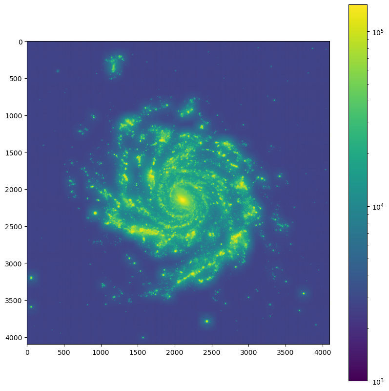
plt.figure(figsize=(10,10))
plt.imshow(hdus[0][1].data, norm=LogNorm(vmin=1e3))
plt.colorbar()

<matplotlib.colorbar.Colorbar at 0x7f4e2b438990>