Wide-field observations of PSF variations with SCAO

In this example we will show the effect of the off-axis AO correction on the shape of the PSF when observing with the SCAO mode. To make a semi-realistic observation, we will observe an open cluster created by the ScopeSim_Templates package. This cluster extends over the full MICADO field of view. As such it should show the full extend of the expected PSF variations over the field.

It should be noted that adding PSF field variations is a computationally expensive process. ScopeSim does it’s best to reduce the level of complexity by discretising the PSF variation into different zones over the field of view. Occasionally the borders between these zones is visible

%matplotlib inline
import datetime
import shutil
import numpy as np
import matplotlib.pyplot as plt
from matplotlib.colors import LogNorm
from astropy import units as u

import scopesim as sim
import scopesim_templates as sim_tp

C:\Users\ghost\AppData\Local\Temp\ipykernel_17984\2683991280.py:10: DeprecationWarning: In a future version top level function calls will be removed. Always use this syntax: from module.submodule import function
  import scopesim_templates as sim_tp

The PSF field-variation is complex and computationally expensive. Hence this functionality is not inluded in the MICADO package. For use cases requireing field variations we must use the pipeline-oriented MICADO package. As we will be using the SCAO mode, we can ignore the MORFEO module.

sim.download_packages(["Armazones", "ELT", "MORFEO", "MICADO"])

Note

In ScopeSim v0.5 both download_packages (new format) and download_package (old format) exist.

If we would like to keep the instrument packages in a separate directory, we can set the following config value:

sim.rc.__config__["!SIM.file.local_packages_path"] = "path/to/packages"

Set up an open cluster Source object

The first step is to create a Source object. Here we take advantage of the cluster function from the ScopeSim_Templates.stellar.clusters submodule. The cluster function draws masses from an standard Kroupa IMF until the mass limit has been reached. It then generates randomly draw positions from a 2D gaussian distribution with a HWHM equal to the given core_radius in parsec. The distance parameter sets the distance in parsec to the centre of the cluster. This allows the final on-sky star positions in units of arcsec from the centre of the cluster to be calculated. Spectra for all the stars are taken from the Pickles (1998) catalogue and are imported from the Pyckles python packages.

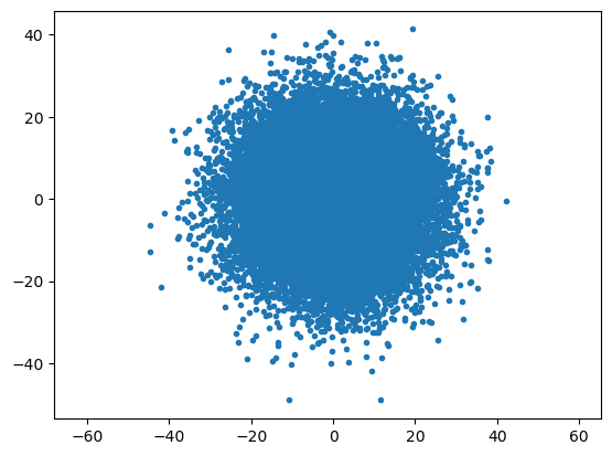
Here we choose a cluster with a mass of 10000 solar masses (~250000 stars) with a core radius of 0.5 parsec, located at a distance of 8 kpc from the Earth. This essentially gives us a cluster that covers the whole MICADO filed of view in wide-field mode (4mas / pixel).

cluster = sim_tp.cluster(mass=10000, core_radius=0.5, distance=8000)

fig, ax = plt.subplots()
ax.plot(cluster.fields[0]["x"], cluster.fields[0]["y"], ".")
ax.set_aspect('equal', 'datalim')

Set up the MICADO optical system for SCAO and include a field-varying PSF

The next step is the standard proceedure - set the instrument to MICADO and the modes to SCAO and IMG_4mas, then create an OpticalTrain object.

observation_dict = {
        "!OBS.mjdobs": datetime.datetime(2022, 1, 1, 2, 30, 0)
}

cmd = sim.UserCommands(
    use_instrument="MICADO",
    set_modes=["SCAO", "IMG_4mas"],
)
micado = sim.OpticalTrain(cmd)

By default the PSF model in the pipeline-oriented MICADO package is set to use a field-constant PSF cube. We need to change this to use a Field-Varying PSF model.

Note: to view all the optical effects contained within the optical model, use the .effects attribute in the OpticalTrain class.

Here we see the PSF model in the 4th last line:

micado.effects

Table length=23

element	name	class	included
str13	str29	str31	bool
armazones	skycalc_atmosphere	SkycalcTERCurve	True
ELT	telescope_reflection	SurfaceList	True
MICADO	micado_static_surfaces	SurfaceList	True
MICADO	micado_ncpas_psf	NonCommonPathAberration	True
MICADO	filter_wheel_1 : [open]	FilterWheel	True
MICADO	filter_wheel_2 : [Ks]	FilterWheel	True
MICADO	pupil_wheel : [open]	FilterWheel	True
MICADO_DET	full_detector_array	DetectorList	False
MICADO_DET	detector_window	DetectorWindow	True
MICADO_DET	qe_curve	QuantumEfficiencyCurve	True
...	...	...	...
MICADO_DET	detector_linearity	LinearityCurve	True
MICADO_DET	border_reference_pixels	ReferencePixelBorder	True
MICADO_DET	readout_noise	PoorMansHxRGReadoutNoise	True
MICADO_DET	source_fits_keywords	SourceDescriptionFitsKeywords	True
MICADO_DET	extra_fits_keywords	ExtraFitsKeywords	True
default_ro	relay_psf	FieldConstantPSF	True
default_ro	relay_surface_list	SurfaceList	True
default_ro	extra_fits_keywords_ro	ExtraFitsKeywords	True
MICADO_IMG_LR	micado_wide_field_mirror_list	SurfaceList	True
MICADO_IMG_LR	micado_adc_3D_shift	AtmosphericDispersionCorrection	False

We can access the PSF model using the standard python dictionary notion using the name of the element. In this case it is called relay_psf as this refers to the internal MICADO relay optics which are connected to the SCAO system.

We do not want to use the default relay_psf object, so we need to tell ScopeSim not to include it

micado["relay_psf"].include = False

Next we want to add a FieldVaryingPSF object from the ScopeSim library of optical effect. Before we initialise the object though, we will need the correct PSF cube.

A small library of precomputed PSFs can be found on the ScopeSim server: https://scopesim.univie.ac.at/InstPkgSvr/psfs/

Once we have downloaded the PSF cube of our choice (in this case the cube corresponding to ESO median atmospheric conditions) we can pass the file path to the FieldVaryingPSF object.

from astropy.utils.data import download_file
fname2 = download_file("https://scopesim.univie.ac.at/InstPkgSvr/psfs/AnisoCADO_SCAO_FVPSF_4mas_EsoMedian_20190328.fits", cache=True)

fname = "AnisoCADO_SCAO_FVPSF_4mas_EsoMedian_20190328.fits"
shutil.copy(fname2, fname)
fv_psf = sim.effects.psfs.FieldVaryingPSF(filename=fname, name="SCAO_FV_PSF")

We now need to add the new PSF to the MICADO relay optics element inside the MICADO optical train.

micado.optics_manager["default_ro"].add_effect(fv_psf)

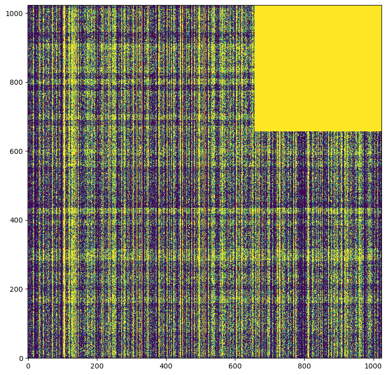
Viewing an on-axis PSF is boring. Therefore we will move the 1024x1024 detector window off centre 10 arcseconds in both x and y directions. We will also increase the exposure time to 60 seconds.

Now we are ready to observe and readout the MICADO detector window

micado.cmds["!OBS.dit"] = 600    # [s]
micado.cmds["!DET.x"] = 10       # [arcsec]
micado.cmds["!DET.y"] = 10

micado.observe(cluster)
hdus = micado.readout()

The elongation of the PSF along the radial axis is quite visible.

!!! It appears

plt.figure(figsize=(20, 20))
plt.subplot(121)
im = hdus[0][1].data
plt.imshow(im, origin="lower", norm=LogNorm(vmin=0.9*np.median(im), vmax=1.1*np.median(im)))

<matplotlib.image.AxesImage at 0x2ed38b526d0>

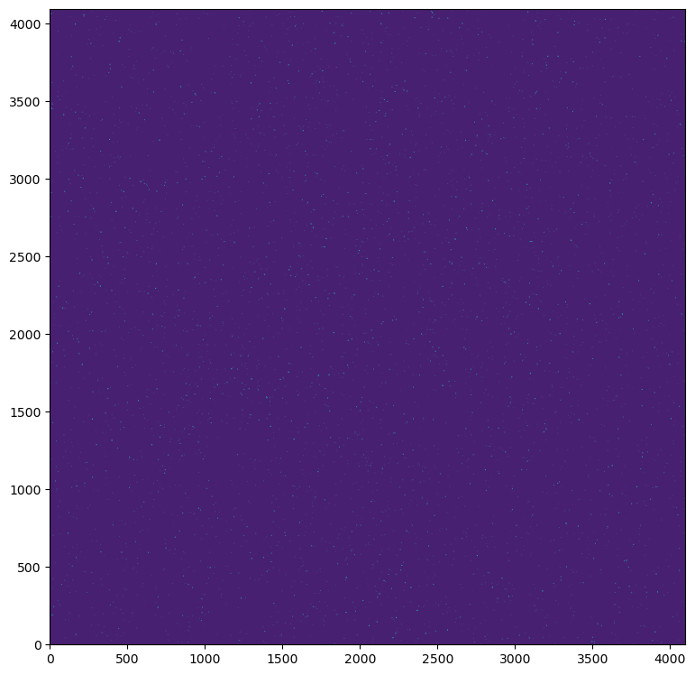
Alternatively we could re-centre the detector window, but expand the window size to 4096x4096 pixels (16x16 arcsecond) which is the equivalent of the central MICADO detector.

micado.cmds["!DET.x"] = 0
micado.cmds["!DET.y"] = 0
micado.cmds["!DET.width"] = 4096
micado.cmds["!DET.height"] = 4096

micado.observe(cluster)
hdus = micado.readout()

It should be noted, the larger the detector size, the longer the simulation takes to run. Hence the option to simply shift the detector centre while keeping the detector size small.

This option does however let us see the change in orientation of the PSF elongation around the on-axis position

plt.figure(figsize=(20, 20))
plt.subplot(121)
im = hdus[0][1].data
plt.imshow(im, origin="lower", norm=LogNorm(vmin=0.9*np.median(im), vmax=3*np.median(im)))

<matplotlib.image.AxesImage at 0x2ed38b9f310>

Swap between a detector window and the full detector array

WARNING! It is ONLY recommended to run the full MICADO detector configuration is you have >8 GB of RAM

While the MICADO package only has a customisable detector window for simulated observations, the MICADO package contains a full description of the 9 detectors in the MICADO detector array.

This requires simulating a ~13000x13000 pixel field, which understandable takes a lot of computer resources and takes on the order of 10 minutes to run.

Ideally the user would write a script using the commands in this notebook and run that script in the background.

That said, swapping to the full detector array is a simple matter of setting the .include parameter to True and False for the two Detector options provided in the MICADO package (see micado.effects table above).

# micado["full_detector_array"].include = True
# micado["detector_window"].include = False

In this case, it is worth saving the final HDUList to disk as a multi-extension FITS file so the data are safe in case something happens to the Python session

# micado.observe(cluster)
# micado.readout(filename="micado_full_detector.fits")